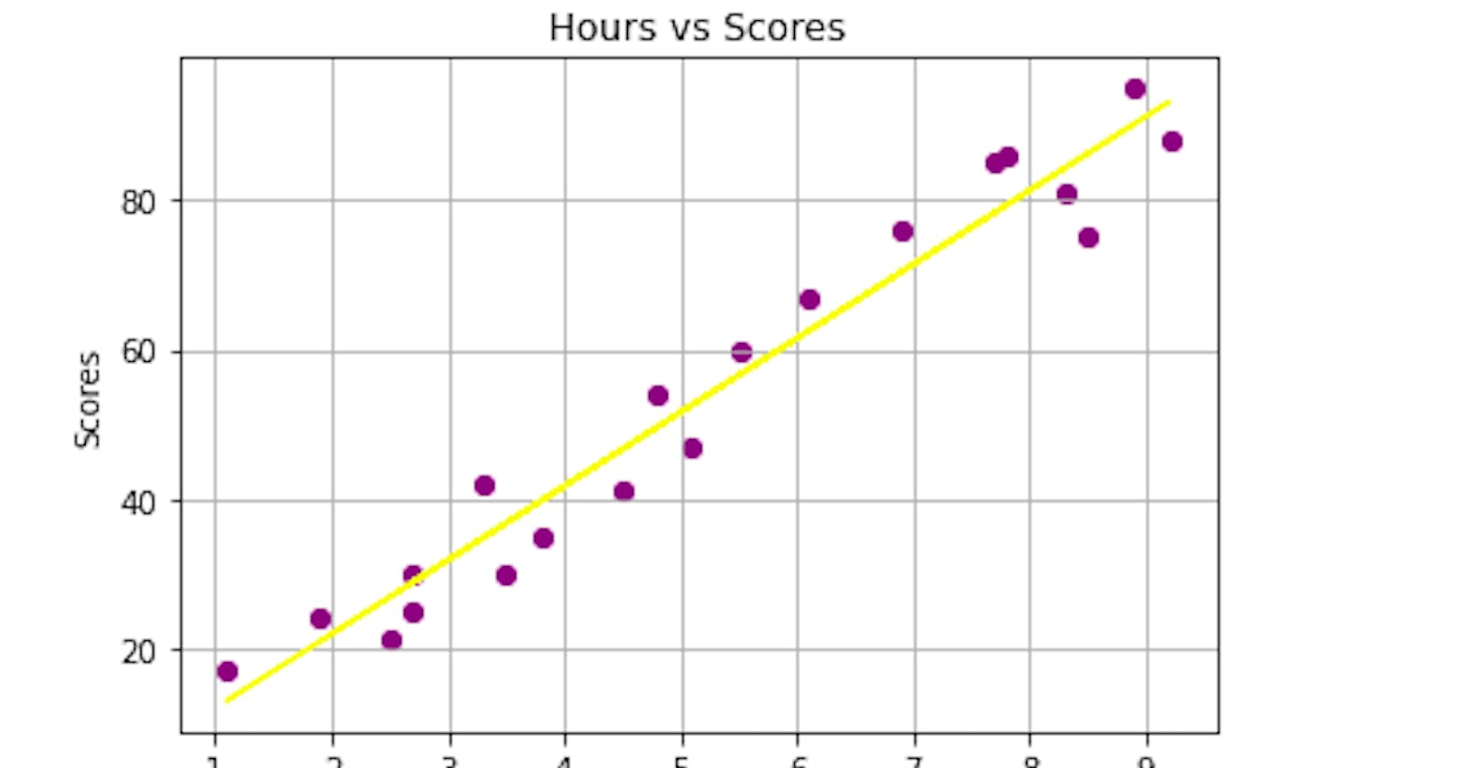
Linear regression is an algorithm that is used to visualize the relationship between two variables. The two variables which are used in this algorithm are the independent and dependent variables.
The independent variable is the variable that is not impacted by the other variable. When adjustments are made in this variable, the levels of the dependent variable will fluctuate.
The dependent variable is the variable that is being studied, and is what the regression model attempts to predict.
The relationship between the input variables (X) which is the dependent variable and the target variables (Y) which is the independent variable is portrayed by drawing a line through the points in the graph. The line represents the function that best describes the relationship between X and Y with the end goal being to find an optimal “regression line”, or the line of best fit.
y(x) = w0 + w1 * x
where:
w = model's parameters.
I will be demonstrating a simple linear regression in this project.
Background:
To identify the correlation of student's scores by the number of hours they study.
Interested parties:
The shareholders that would be interested in this project includes; the school administrators, education ministries and students.
Data:
The data contains the number of hours of study of each student and their respective scores.

Checking the statistical information, the mean hour was 5. 0 with the mean score being 51.5

Visualization:
Using lmplot, a visualization style from seaborn to show what the dataset looks like.

Model Building:
Using linear regression from scikit-learn to build and train this model, which splitting the dataset with the parameters of 80% training and 20% test with a random state of 0.
After training, I visualized the prediction of the model

Making a comparison between the actual values and predicted values and checking their correlation.


Testing the prediction of my model with the score of a student that studies for 9.25 hours.

Mean Absolute Error:
This is the results of measuring the difference of two continuous variables. This measurement is done by taking the absolute value of each error and getting its average.
For my project, the MAE is 4.183
Mean Square Error:
This is average of the difference between the estimated value and the actual value. This is calculated by taking the average of the square of the difference between the original and predicted values of the data.
For my project, the MSE is 21.60 which is quite high.
Root Mean square Error:
This is the standard deviation of the errors which occur when a prediction is made on a dataset.
My project has the RMSE of 2.05
Finally, the accuracy of prediction of my model was 95%.
Conclusion:
This is a project from my TSF participation. The code to this project can be found in my repo and you can connect with me on LinkedIn . All suggestions, corrections and recommendations are really appreciated. Thank you for reading.
