Background:
Introduction of artificial intelligence into the healthcare has revolutionized the industry. In terms of magnetic resonance imaging(MRI), it has produced faster and better tumor and cancer detection with segmentation and localization.
Problem statement:
As an AI/ML consultant, a medical diagnostic company has tasked you with the improvement of the speed and accuracy of detecting and localizing brain tumors based on MRI scan. The dataset provided contains 3929 brain MRI scan with their tumor location for you to develop a model that detects and localizes brain tumors.
Interest:
The interest of this company is to increase early diagnosis of brain tumors and reduce cost of cancer diagnosis.
Solution:
To solve the above problem, a classification and segmentation model is built.
Data:
Source:
The data is sourced from here
Using the .info function, I printed the columns in the csv file

Then with the .head function, I printed the first 30 rows in the dataset


As seen in the above, the column named mask has a value of 0, indicating the absence of tumors.
Data Visualization
Using matplolib.pyplot, I visualized the 723rd image in the dataset which has a max of 255 and a min of 0.

Then using the random function, I visualized six brain MRIs which generated both MRIs with tumors and those without tumors.


Splitting:
Using the train_test_split function, I split the data into training and testing with value of 15%. Then using data image generator from keras, I rescaled the data and made a validation data split of 15%.
Data generation:
I generated the train, validation and test image generation subsets with batch size of 16, class mode which equals categorical and target size as (256,256) with shuffle equals false.

I created a base model with resnet50 with weights from a pretrained value which is the imagenet. Below is the summary of the base model.

Building network:
I built the network using two hidden layers with activation relu, dense of 256 and a dropout of 0.3 with the output layer using the softmax activation. Below is the model summary.

Compilation:
I compiled the model using categorical crossentropy for loss, adam optimizer and ‘accuracy’ metrics.
I also used early stoppage after a patience of 20, with checkpoints setting the save_best_model to true. Training:
This is where there was trial and error. The first model was trained with 10 epochs which resulted in the accuracy of 0.329 with this visualized confusion metrics.

 Model 1
The second model was trained with 50 epochs. the training didn’t get to the 50 epochs as the early stoppage was triggered resulting the model to stop at 33 epochs. This model had an accuracy of 0.866, couldn’t work on its visualized confusion metrics.
 Model 2
The third model was trained with 1 epoch with some of the hyperparameters changed. The validation was split to 20% instead of 15%. The accuracy was at 0.76 with this visualized confusion metrics.

 Model 3
The final model was trained with 25 epochs which had the accuracy of 0.946 and this visualized confusion metrics.

 Model 4
Looking at the models above, we have our winner, the fourth model.
Score:
Using the scikit learn classification_report function, the image below was the report.

Segmentation model:
The segmentation model which will help in the localization was built using mask which its goal is to understand the image at pixel level.
Methodology:
The data was split into train, validation and test subsets. Loss function was done using a custom loss function which is the Tversky loss function. You can read up more about it here and the repo of the function can be found here. Adam optimizer was used with a learning rate of 0.05 and epsilon of 0.1, loss function of focal_tversky and the ‘tversky’ metrics. Early stoppage and checkpoints were also applied.
Training:
The segmentation model was trained using 10 epochs with loss of 0.19 and tversky of 0.88


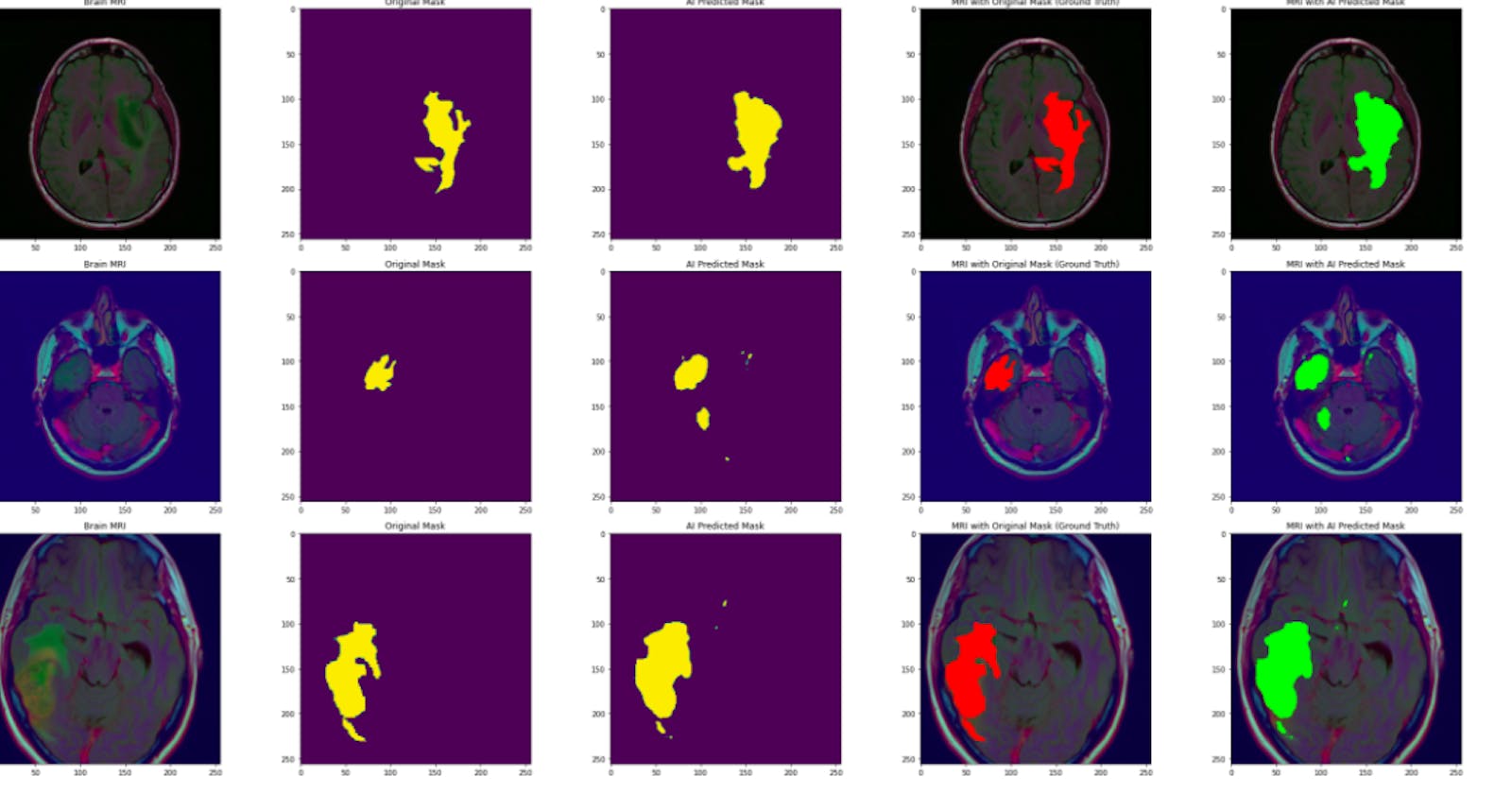
The result of the above isn’t sufficient for segmentation as a false negative was seen.

Visualization:
The model was plot to visualize MRIs with the scan, original mask, predicted mask, ground truth and scan with the predicted mask.


Discussion:
The reason for training different models was to get a higher accuracy and eliminating false positives and false negatives. This helps eliminate misdiagnosis.
Conclusion:
All models combined took 48 hours to train and it was my first time bumping into the tversky function. Any suggestion on how to improve the accuracy of this model to at least a 99% is welcomed, you can reach me through my LinkedIn profile.
PS: This is a part of my certification course I took in Udemy.
